Section 6.2: Gain and Antenna Patterns #

An antenna’s quoted gain tells only part of the story. A large number is little comfort if the other station sits in a null, or if a strong noise source falls in a side lobe. The radiation pattern shows where the antenna’s gain will help and where it will not.

The pattern also shows where that gain comes from: an antenna concentrates power in some directions by taking it from others. Like a squeezed balloon, it can only bulge out where it’s pinched in somewhere else.

Key Information: There is no difference in radiated power between a lossless antenna with gain and an isotropic radiator driven by the same power.

Reading the Free-Space Pattern #

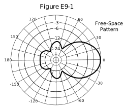
Figure E9-1 is a polar plot. Angles run around the outside; distance from the center represents relative signal strength in decibels. The outer edge is the peak reference, 0 dB. The thick curve traces the antenna’s response. The spokes are 15 degrees apart. Inward from the unlabeled 0 dB edge, the labeled rings are −3, −6, −12, and −24 dB. Their decibel steps differ, so check the labels before estimating a level between rings.

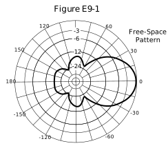
Figure E9-1, a free-space antenna pattern plotted on a circular decibel grid, with spokes every 15 degrees and labeled rings at minus 3, minus 6, minus 12, and minus 24 dB inside the zero-dB outer edge. The main lobe points right at zero degrees and peaks at the outer reference circle. Its minus-3-dB crossings are near plus and minus 25 degrees, giving a 50-degree beamwidth. Response directly behind at 180 degrees is about 18 dB below the forward peak. The side response near plus or minus 90 degrees is about 14 dB below the peak. Smaller side and rear lobes show that the antenna also radiates away from its main direction. — Figure E9-1: Direction and relative strength in a free-space pattern.

The broad outward bulge toward zero degrees is the main lobe. Smaller bulges are side or rear lobes. To find the 3 dB beamwidth, locate where the main lobe crosses the $-3$ dB circle on each side of its peak. Those points are about $+25^\circ$ and $-25^\circ$ , so the full width is $25-(-25)=50^\circ$ , not the 25 degrees from the peak to one side. At each point, power density falls to half the peak value.

Front-to-back ratio compares the forward peak with the response directly behind it. Front-to-side ratio compares the forward response with the response 90 degrees to the side. Read each level on the decibel grid, then subtract it from the 0 dB peak. At 180 degrees, the curve sits roughly halfway between the −12 and −24 dB rings, at about −18 dB, so the front-to-back ratio is $0-(-18)=18$ dB. At 90 degrees, the curve lies a little inside the −12 dB ring, at about −14 dB.

Key Information: For the antenna radiation pattern shown in Figure E9-1:
The 3 dB beamwidth is 50 degrees.
The front-to-back ratio is 18 dB.
The front-to-side ratio is 14 dB.

Looking Above the Horizon #

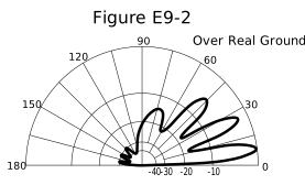
A bearing around the horizon does not tell us whether the strongest lobe points low or nearly overhead. An azimuth pattern gives the horizontal slice; an elevation pattern shows radiation at different angles above the horizon. Figure E9-2 includes the ground, so only the upper half of the circle appears.

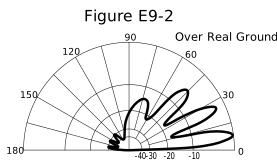
Figure E9-2, an elevation radiation pattern over real ground. The horizontal baseline is the horizon, with forward zero degrees to the right, 90 degrees overhead, and the rear horizon at 180 degrees to the left. The strongest forward lobe peaks only about 7.5 degrees above the horizon. Other weaker forward lobes rise at higher angles, separated by deep nulls. Small rear lobes are about 28 dB below the strongest forward response. Concentric rings, labeled along the forward baseline, show minus 10, minus 20, minus 30, and minus 40 dB. — Figure E9-2: Elevation lobes produced over real ground.

The longest lobe hugs the right-hand horizon. Its peak lies halfway between zero and 15 degrees. This plot uses a different level scale: labels along the right-hand baseline mark its rings at −10, −20, −30, and −40 dB. Follow those rings around to the rear lobes. They reach just outside the −30 dB ring, toward the edge, about 28 dB below the forward peak at 0 dB.

Key Information: For the radiation pattern shown in Figure E9-2:
It is an elevation pattern.
The elevation angle of peak response is 7.5 degrees.
The front-to-back ratio is 28 dB.

A Modeled Pattern #

Antenna-modeling software often calculates patterns like these and also predicts feed point impedance. It divides each wire into short pieces called segments, solves for the current in each, and combines the fields they produce. The Method of Moments turns these field relationships into equations a computer can solve.

Current changes along a real wire, so each segment must be short enough for a single value to stand in for its part of the wire. With too few segments, the model can’t follow those changes.

Key Information:
Method of Moments analysis is commonly used for modeling antennas.
The principle of a Method of Moments analysis is that a wire is modeled as a series of segments, each having a uniform value of current.
A disadvantage of decreasing the number of wire segments in an antenna model below 10 segments per half-wavelength is that the computed feed point impedance may be incorrect.

Some programs give each segment a more detailed current shape, but the same limit applies. More segments cannot repair wrong wire dimensions, missing conductors, or an unsuitable ground model. Before trusting a beautiful plot, check what you told the model about the actual antenna and its surroundings.

Naming the Gain Reference #

Whether a gain figure comes from a model or a catalog, check its reference. dBi compares an antenna with an isotropic radiator; dBd compares it with a half-wave dipole in free space. The dipole’s maximum gain is 2.15 dBi, so convert with

G_{\text{dBd}}=G_{\text{dBi}}-2.15.

Key Information: An antenna with 6 dB gain over an isotropic radiator has $6-2.15=3.85$ dB gain compared to a half-wavelength dipole.

Power After Losses and Gain #

The same two references carry into power calculations. Effective radiated power, or ERP, describes a system’s signal in one direction. It is the power a lossless half-wave dipole would need to produce the same signal there. Effective isotropic radiated power, or EIRP, uses the isotropic reference instead. Neither one is power summed over all directions. Because the antenna concentrates its radiation, either can exceed the transmitter’s output.

Key Information: Effective radiated power is the term describing total radiated power that takes into account all gains and losses.

Add the gain and subtract losses in decibels first. Then convert the net decibel change to a power multiplier:

P_{\text{equivalent}}=P_{\text{transmitter}}\times10^{G_{\text{net}}/10}.

A duplexer, which lets a repeater share an antenna between transmitter and receiver, adds insertion loss. A circulator, which routes RF between ports in a fixed sequence, can add loss too. Subtract each loss between transmitter and antenna once.

For a 150-watt transmitter, 2 dB line loss, 2.2 dB duplexer loss, and 7 dBd antenna gain,

G_{\text{net}}=7-2-2.2=2.8\text{ dB},

ERP=150\times10^{2.8/10}\approx286\text{ W}.

Use the calculator’s $10^x$ function: $10^{0.28}\approx1.91$ , so the net change multiplies 150 watts by about 1.91. The other examples use the same steps:

Reference and transmitter	Net gain after losses	Equivalent power
ERP, 200 W	$10-4-3.2-0.8=2$ dB	$200\times10^{2/10}\approx317$ W
EIRP, 200 W	$7-2-2.8-1.2=1$ dB	$200\times10^{1/10}\approx252$ W

Key Information:
A repeater station with 150 watts transmitter power output, 2 dB feed line loss, 2.2 dB duplexer loss, and 7 dBd antenna gain has an effective radiated power (ERP) of 286 watts.
A repeater station with 200 watts transmitter power output, 4 dB feed line loss, 3.2 dB duplexer loss, 0.8 dB circulator loss, and 10 dBd antenna gain has an ERP of 317 watts.
A repeater station with 200 watts transmitter power output, 2 dB feed line loss, 2.8 dB duplexer loss, 1.2 dB circulator loss, and 7 dBi antenna gain has an effective isotropic radiated power (EIRP) of 252 watts.